The authors train \(m\) different VAEs that learn to compress the spherical harmonics (SH) volume representing the fODFs. Each \(m_i\) VAE learns a latent representation of a different coefficient of the fODF map.
The encoder \(\mathcal{E}^{(i)}\) will learn to compress the \(i^{th}\) coefficient of the fODF map into a latent space \(z^{(i)}\).
2. Training the Generative model (Diffusion or Flow Matching) #
They first create a global conditioning tensor \(z\) by fusing and refining each \(z^{(i)}\) produced by the VAEs:
The \(\mathcal{E}^c\) is a 3D ResNet that refines the vectors \(z^{(i)}\) from the VAEs: \(\hat{z}^{(i)} = \mathcal{E}^c (z^{(i)}, i)\). Its weights are shared across all VAE outputs and are conditioned on \(i\) to inform of the coefficient specific context.
The final global conditioning tensor \(z\) is created by flattening and concatenating, channel-wise each \(\hat{z}^{(i)}\).
\(\mathcal{E}^c\) is trained jointly with the following steps for the generative model.
They then train the core generative model, which is based on a conditional transformer:
Model receives inputs:
Noisy streamline \(x_t\) of shape (p, 3)
Timestep \(t\)
Global context tensor \(z\)
M stacks of Transformer models with following attention mechanisms
Self-attention: to insure internal coherence between each streamline points.
Cross-attention: to integrate context from the global context \(z\). To enable cross-attention, the authors linearly project the \(z\) and \(x_t\) to an embedding space of same dimension \(n\) (128, 256 or 512).
Transformer trained to remove noise from the initially noisy streamlines. Depending on their experiment (although the final model ends up being the diffusion objective), they use two different objectives:
\(L_{D}(\theta) = E_{t, x_0, \epsilon} [||\epsilon_{\theta}(x_t, t) - \epsilon||^2]\). Which aims to learn to predict the noise to remove from the noisy streamline.
\( L_{FM}(\theta) = E_{t, x_0, x_1}[||v_{\theta}(x_t, t) - v||^2] \) where \(v=x_1 - x_0\). It essentially aims to learn to directly predict the vector field associated with the change between two time steps of the reverse diffusion process.
For training, the authors use the 1042 subjects from HCP Young Adult dataset (age 22-35). The HCP data is downsampled to \(1.875mm^3\) isotropic and the SH coefficients are z-score normalized.
They use the PyAFQ tractography pipeline to generate tractograms to train the model.
PyAFQ generates tractograms either using a probabilistic tractography algorithm or particle filtering tractography (PFT).
Gold standard: PyAFQ registers the subject’s data to a template and uses its own filtering pipeline to filter streamlines based on geometric plausibility and alignment with the atlas’ predefined 24 known bundles (waypoint-based method or Recobundles).
Training set is augmented by rotating the SH volume and its corresponding tractogram deterministically (15, 30, 45 degrees).
Practically, all streamlines coordinates are scaled to [-1, 1].
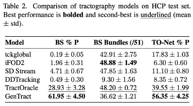
Authors use the HCP (test set containing 15% of the data) with full resolution as a baseline comparison.
They test models in more challenging conditions:
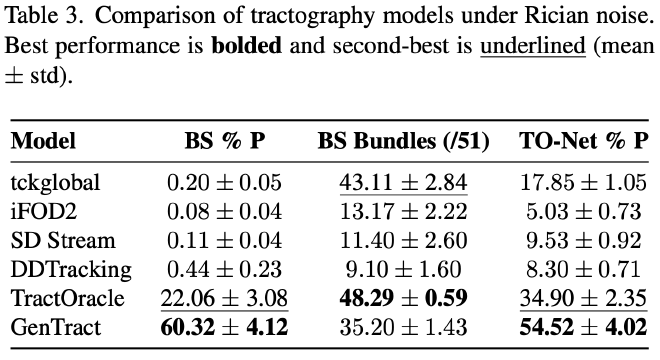
They add Rician noise (\(\sigma = 0.005\)) to the DWIs of the test set.
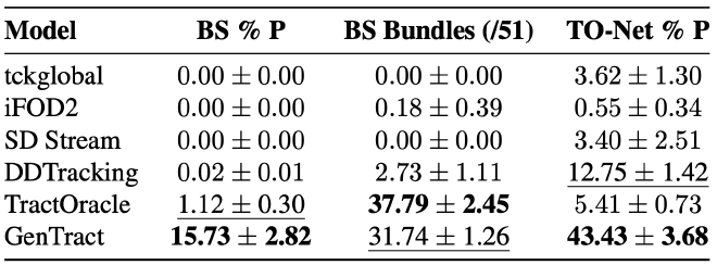
They add Rician noise (\(\sigma = 0.005\)) to the DWIs and downsample the HCP test set to \(3mm^3\) isotropic to simulate low-field clinical data.
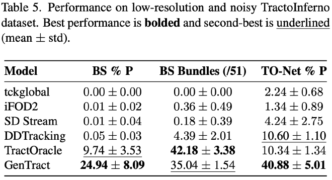
They test on TractoInferno which they synthetically downsample to \(3mm^3\) isotropic and add Rician noise (to evaluate on an external dataset).
Metrics
Precision: \(\frac{TP}{TP+FP}\). Higher value indicates that the model generates a high rate of valid streamlines and avoids generating invalid streamlines. They compute precision 3 ways:
BS % P: BundleSeg precision (when comparing with SOTA tractography algorithms).
TO-Net & P: TractOracleNet precision.
Number of discovered bundles (/24)
Inference time: mean wall-clock time to generate a full tractogram.
Results
Authors evaluate the difference in performance between choosing between a flow matching (FM) approach and a diffusion approach with varying number of layers (\(M={4, 6, 8}\)) and different embedding layer sizes (\(n={128, 256, 512}\))
The diffusion network with \(M=8\) and \(n=256\) gave better AFQ % P.
They also conclude that 10 DDIM inference steps during inference gave the best compromise between computational demand and performance.
Performance on HCP (raw)
Performance on HCP (Rician noise)
Performance on HCP (Rician noise + downsampling)
Performance on TractoInferno (Rician noise + downsampling)The authors also note that the computation time for GenTract is comparable to TractOracle and DDTracking (slightly slower than both), while still being orders of magnitude faster than other methods.